Flory-Huggins Lattice Theory
of Polymer Solutions, Part 2

The classical thermodynamics of (binary) polymer solutions was first developed by Paul Flory¹ and Maurice Huggins² independently in the early 1940s. They assumed a rigid lattice framework and a regular solution (random mixing) and obtained for the free energy of mixing per unit volume following expression:

Δf_mix / kT = φ_p / (r·v_r) · ln φ_p + φ_s / v_s · ln φ_s + χ_ps φ_s φ_p / v

where φ_s and φ_p are the volume fractions of the solvent and polymer,

φ_s = N_sv_s / (N_sv_s + N_prv_r),   φ_p = N_prv_r / (N_sv_s + N_prv_r)

The two parameters v_s and v_r are the volumes of a solvent molecule and of a polymer repeat unit with one and r repeat units respectively. The parameter v is the average segmental volume, (v_rv_s)^1/2.

Assuming equal lattice volumes for both repeat units, as was assumed by Flory¹, the free energy per lattice site can be written as

Δf_mix / kT ≈ φ_p / r · ln φ_p + φ_s ln φ_s + χ_ps φ_s φ_p

At first it was assumed that the interaction parameter χ is independent of the concentration φ_p. But it became soon evident that χ is a function of both the temperature T and concentration of the polymer. Furthermore, χ is also a function of the molecular weight of the polymer, not only at low but also at high polymer concentrations. However, there are quite a number of cases where χ seems to be independent of composition, i.e. good solvents,  as was proposed by the original Flory-Huggins theory. Some examples are polyisobutylene (PIB) in cyclohexane and poly(dimethyl siloxane) (PDMS) in n-octane. For this situation, the prediction of the free energy of mixing and of the phase curves (binodal and spinodal) is least difficult.

 

Temperature Dependence of Interaction Parameter

The temperature dependence of the interaction parameter is quite obvious from the definition of the χ parameter:

χ(T) = -z/2 (ε_pp + ε_ss - 2 ε_ps) / kT = B / T

where B describes the temperature dependence of χ. According to this equation, χ is a linear function of the inverse temperature. For the case B > 0 and (very) low temperatures, the free energy curve is concave and homogenous mixtures are unstable because the second derivative of the free energy of mixing is negative and the contribution of the entropy is small.

In most cases, mixing of a polymer with a solvent results in a volume change, that is, local packing effects lead to a temperature-independent additive constant in the Flory expression for the interaction parameter. Empirically, the temperature dependence of χ is often written as a sum of two terms:

χ(T) = A + B / T

The temperature independent term A is the so-called "entropic part" of of χ, while B / T is called the "enthalpic part". The parameter A and B have been tabulated for many polymer-solvent and polymer-polymer systems.

Binodal Phase curve

The phase boundary between the single- and two-phase region, the so-called binodal, can be determined from the common tangent of the free energy of mixing at the compositions φ_P,B¹ and φ_P,B², corresponding to the equilibrium composition of the two phases:

∂Δf_mix / ∂φ_P |φ_P,B¹ = ∂Δf_mix / ∂φ_P |φ_P,B^2-

The derivative of Δf_mix is

∂Δf_mix / ∂φ_P = kT · [r ^-1 ln φ_p + r^-1 - ln φ_s - 1 + χ (1 - 2φ_p)]

 

And for the general case of two polymers with r and s repeat units per polymer:

∂Δf_mix / ∂φ_p1 = kT · [r ^-1 ln φ_p1 + r ^-1 - s^-1 ln (1-φ_p1) - s^-1 + χ (1 - 2φ_p1)]

For the simple case of polymers of equal length, r = s = n, the tangent is horizontal:

∂Δf_mix / ∂φ_p1 = kT · [n ^-1 ln φ_p1 - n^-1 ln (1-φ_p1) + χ (1 - 2φ_p1)] = 0

This equation can be solved for the Flory-Huggins parameter corresponding to the binodal (phase boundary):

n · χ_B = ln φ_p1 - ln (1-φ_p1) / (1 - 2φ_p1) = ln [φ_p1 / (1-φ_p1)] / (1 - 2φ_p1)

And with the temperature dependence of the interaction parameter, χ = A + B / T, this relation can be solved for the binodal of the phase diagram, i.e. for the binodal temperature as a function of composition:

T_B = B / {ln[φ_p1 / (1 - φ_p1)] / (2 n φ_p1 - n) - A}

 

Spinodal Phase Curve

The boundary between the unstable and metastable region, the so-called spinodal, can be calculated from the inflection points of the free energy curve:

(∂²Δf_mix / ∂φ_P²)_p,T = kT {(φ_p r)^-1 + [(1 - φ_p) s]^-1 - 2χ} = 0

This equation can be solved for the Flory-Huggins interaction parameter corresponding to the spinodal phase boundary:

χ_S = ½ {(φ_p r)^-1 + [(1 - φ_p) s]^-1}

The spinodal phase boundary can also be written as a temperature-composition relation:

T_S = B / {(2φ_p r)^-1 + [2(1 - φ_p) s]^-1 - A}

In a binary blend, the lowest point of the spinodal corresponds to the critical point⁴:

χ_c = ½ · (r ^-½ + s^-½)²

or

T_c = B / (χ_c - A) = B / {½ · (r ^-½ + s^-½)² - A}

For a symmetrical polymer mixture, r = s = n, the whole phase curve becomes symmetric with the critical point:

χ_c = 2 / n  and  φ_c = 1/2

whereas in polymer solutions, r = n and s = 1, the whole phase curve becomes very asymmetrical with the critical point:

χ_c ≈ ½ + 1 / n^½  and  φ_c = 1 / n^½ 

Spinodal and Binodal Phase Diagram

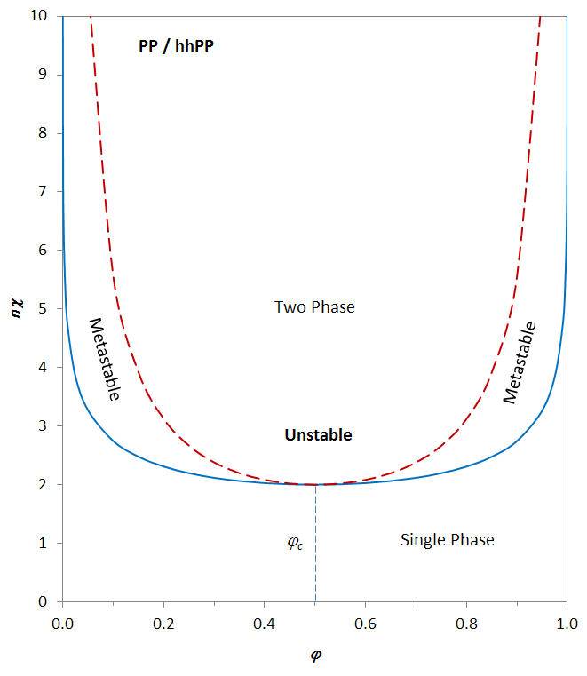
The figure above shows the product n χ as a function of polymer concentration φ_p for a symmetrical blend of polypropylene (PP) and head-to-head polypropylene (hhPP). The binodal (solid curve) and spinodal (dashed curve) have been calculated with the equations above and the parameters A = -0.0036 and B = 1.84. The two curves coincide at the critical point.

References and Notes

1. P. J. Flory, J. Chem. Phys. 9, 660 (1941); 10, 51 (1942)
2. M. L. Huggins, J. Phys. Chem. 46, 151 (1942); J. Am. Chem. Soc. 64, 1712 (1942)
3. Paul L. Flory, Principles of Polymer Chemistry, Ithaca, New york, 1953
4. Note, the spinodal and binodal of any binary mixture meet at the critical point.